今天补充一些有关均值方差的公式和高斯分布的一些性质。

Some Formulas of Mean and Variance

定理一： We consider two random variables $X$ and $Y$

定理二： When $X$ is indenpendent of $Y$

定理三： For $n$ random variables $X_1,…,X_n$

where $E(X_i)=\mu_i$ and $a_i$ is a constant value. When $X_1,…,X_n$ are mutually independent, we have the following:

Transformation of Variables

When a distribution of $X$ is known, we can find a distribution of $Y$ using the transformation of variables, where $Y$ is a function of $X$.

定理四： Distribution of $Y = \phi^{(-1)}(X)$: Let $f_x(x)$ be the pdf of $X$ and $X=\phi(Y)$ be a one-to-one transformation, then the pdf of $Y$ is given by

Example: $X\sim N(0,1),Y = \mu + \sigma X$

Since we have

$$ X = \phi(Y) = \frac{Y-\mu}{\sigma},f_x(x)=\frac{1}{\sqrt{2\pi}}exp(-\frac{1}{2}x^2) $$

then $\phi’(y)=1/\sigma$

which indicates the normal distribution with mean $\mu$ and variance $\sigma^2$, denoted by $N(\mu,\sigma^2)$.

Multivariate Case

Let $f_x(x_1,…,x_n)$ be a joint pdf of $(X_1,…,X_n)$, and a one-to-one transformation from ($X_1,…,X_n$) to ($Y_1,…,Y_n$) is given by

then we obtain a joint pdf of $Y_1,…,Y_n$

where $J$ is the Jacobian of the transformation.

Gaussian Distribution

极大似然估计

说起高斯分布大家都很熟悉了，假设一个 $p$ 维变量 $x \in R^p$ 满足高斯分布 $N(\mu,\Sigma)$，则其概率密度函数可以表示为

当有样本数据 $X_{N \times p}=(x_1,…,x_N)^T$ 时，我们能通过极大似然法估计高斯分布的均值和方差，即

假设 $x_i$ 服从独立同分布 (i.i.d)，则

为了便于计算假设 $p=1$ 且真实高斯分布为 $N(\mu,\sigma^2)$，通过极值条件 (令导数为0) 可以得到

其中,

均值是无偏估计 $E(\mu_{MLE}) = \mu$

方差是有偏估计 $E(\sigma_{MLE}^2)=\frac{N-1}{N}\sigma^2$，也就是说极大似然估计出来的高斯分布的方差是偏小的。

从概率密度函数的角度看高斯分布

注意到高斯分布的概率密度函数 $p(x)$ 本质是关于 $x$ 的函数，且和 $x$ 有关的部分为：

一般来说 $\Sigma$ 是半正定矩阵，为了便于分析其性质，这里假设其为正定矩阵，对其进行特征值分解：

其中，$U=(u_1,…,u_p),UU^T=U^TU=I,\Lambda=diag(\lambda_i)$

则方差矩阵的逆为

定义 $y_i=(x-\mu)^Tu_i$，可以将 $y_i$ 看作是 $x$ 去均值后在向量 $u_i$ 上的投影，则 $\Phi$ 可以表示为

为了便于展示我们取 $p=2$，并令 $\Phi=1$ 可以发现

竟然是一个椭圆！

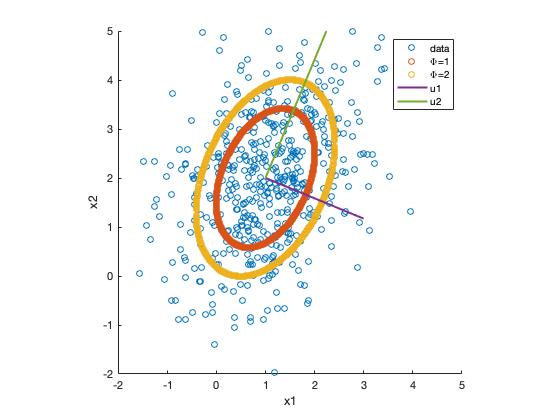
也就是说指定了 $\Phi$ 的值，相当于能够得到高斯分布的等高线。

Matlab code

 1
 2
 3
 4
 5
 6
 7
 8
 9
10
11
12
13
14
15
16
17
18
19
20
21
22
23
24
25
26
27
28
29
30
31
32
33
34
35
36
37
38
39
40
41
42
43
44
45
46
47
48
49
50
51
52
53
54
55
56
57
58
59
60

 clear;
 clear all;
 clf

 mu = [1,2];
 Sigma = [1,0.5;0.5,2];
 X = mvnrnd(mu,Sigma,500); % 从高斯分布中生成样本
 scatter(X(:,1),X(:,2))
 [U,Lambda] = eig(Sigma)；
 u1 = U(:,1); % 对应博客中的投影向量
 u2 = U(:,2);
 lambda1 = Lambda(1,1); % 对应博客中的椭圆长短轴
 lambda2 = Lambda(2,2);

 X1 = [];
 X2 = [];
 % 采用暴力搜索来获取使得\Phi = 1的横纵坐标
 for x1 = -3:.01:5
     for x2 = -4:.01:5
         phi = (([x1,x2] - mu)*u1)^2/lambda1 + (([x1,x2] - mu)*u2)^2/lambda2;
         if phi <= 1.01 && phi >= 0.99
             X1 = [X1;x1];
             X2 = [X2;x2];
         end
     end
 end
             
 hold on 
 scatter(X1,X2)

 X1 = [];
 X2 = [];
 % 采用暴力搜索来获取使得\Phi = 2的横纵坐标
 for x1 = -3:.01:5
     for x2 = -4:.01:5
         phi = (([x1,x2] - mu)*u1)^2/lambda1 + (([x1,x2] - mu)*u2)^2/lambda2;
         if phi <= 2.01 && phi >= 1.99
             X1 = [X1;x1];
             X2 = [X2;x2];
         end
     end
 end
             
 hold on 
 scatter(X1,X2)

 % 画出投影向量
 x = 1:2:3;
 k1 = u1(2)/u1(1);
 k2 = u2(2)/u2(1);
 y1 = k1*(x-mu(1))+mu(2);
 y2 = k2*(x-mu(1))+mu(2);
 plot(x',y1','LineWidth',2)
 plot(x',y2','LineWidth',2)
 xlim([-2, 5]);
 ylim([-2, 5]);
 axis square
 legend('data','\Phi=1','\Phi=2','u1','u2')
 xlabel('x1')
 ylabel('x2')

高斯分布的局限性

1. 协方差矩阵 $\Sigma$ 中的参数个数太多 $p(p+1)/2 = O(p^2)$；可以采用对角化或各向同性的假设。

2. 单高斯分布来拟合数据不合理；可以采用混合高斯模型。

已知联合概率求边缘概率和条件概率

已知

求 $p(x_a),p(x_b|x_a)$。可以采用配方法(见PRML，过于复杂)，这里采用构造定义法。

定义 $A = (I_m \quad 0)$，则 $x_a = Ax$

所以边缘概率分布为

定义

则 $x_{b.a}=Ax$

则可以得到 $x_{b.a}$ 的分布，又因为

条件分布的均值和方差可以表示为

因此条件概率分布为

已知边缘概率和条件概率求联合概率

已知

求 $p(y),p(x|y)$

定义 $y=Ax+b+\epsilon,\epsilon \sim N(0,L^{-1})$

则 $y$ 的边缘概率为

即

要求 $p(x|y)$ 可以构造联合分布，在利用联合概率求条件概率

构造

也就是只要求出 $x$ 和 $y$ 之间的协方差 $\Delta$ 就能够知道它们的联合分布了。根据协方差的定义来求解

这样完整的联合分布就得到了，代入上一节 $x_b|x_a$ 的公式即可得到 $p(x|y)$ 的概率分布了。